This is a short example of how we can use knn algorithm to classify examples. In this article I’ll be using a dataset from Kaggle.com that unfortunately no longer exists. But you can download csv file here : data. This is a dataset of employees in a company and the outcome is to study about employee’s attrition.
Basically, it is a very simple dataset : no missing values, small skewness of data, 5 quantitative features and 2 categorical variables. Each employee is represented by 7 features, and then labelled 1 or 0, depending on if the person left or stayed in the company. Goal of this study is to build a model using knn algorithm which predict the risk of attrition for each employee. In this article I’ll be doing my own implementation of knn and compare it to scikit-learn library solution. This is just a rapid solution to play with knn algorithm and not a complete data analysis, machine learning project.
Dependencies
|
1 2 3 4 5 6 7 8 |
import numpy as np import pandas as pd import math import matplotlib.pyplot as pyplot from sklearn import preprocessing,model_selection from collections import Counter import os import seaborn as sns |
Data loading
using pandas to load csv file and separating X (inputs values) and y (labels). Features values have different ranges, and it will be a problem when calculating distances (as one feature will have a big impact on the distance whereas other will only have a small impact). To normalize the data feature wise between 0 and 1 is a possible solution.
|
1 2 3 4 5 |
df=pd.read_csv('data/data.csv',sep=";") X=np.array(df.drop(['left'],1)) X=preprocessing.normalize(X) y=np.array(df['left']) |
I also prepare subsets of the dataset in our to be able to test the performance of our model. Scikit-learn library does have function for this. We just need to import the train_test_split function from model_selection.
|
1 |
from sklearn import preprocessing,model_selection |
Dataset description
Our dataset in composed of 14999 employees represented by 7 features : satisfaction_level, last_evaluation, number_project, average_montly_hours, time_spend_company, work accident, promotion_last_5years. Each employee is then labeled in the “left” column. 1 if he left the company, 0 if he stayed.
Data analysis and visualization
Let’s start with a small statistical description of the data.
|
1 |
print(df.describe()) |
|
1 2 3 4 5 6 7 8 9 10 11 12 13 14 15 16 17 18 19 20 21 22 23 24 25 26 27 28 29 |
satisfaction_level last_evaluation number_project \ count 14999.000000 14999.000000 14999.000000 mean 0.612834 0.716102 3.803054 std 0.248631 0.171169 1.232592 min 0.090000 0.360000 2.000000 25% 0.440000 0.560000 3.000000 50% 0.640000 0.720000 4.000000 75% 0.820000 0.870000 5.000000 max 1.000000 1.000000 7.000000 average_montly_hours time_spend_company Work_accident \ count 14999.000000 14999.000000 14999.000000 mean 201.050337 3.498233 0.144610 std 49.943099 1.460136 0.351719 min 96.000000 2.000000 0.000000 25% 156.000000 3.000000 0.000000 50% 200.000000 3.000000 0.000000 75% 245.000000 4.000000 0.000000 max 310.000000 10.000000 1.000000 promotion_last_5years left count 14999.000000 14999.000000 mean 0.021268 0.238083 std 0.144281 0.425924 min 0.000000 0.000000 25% 0.000000 0.000000 50% 0.000000 0.000000 75% 0.000000 0.000000 max 1.000000 1.000000 |
Apparently there are no features with missing values which is confirmed by the following command:
|
1 |
print(df.isnull().any()) |
|
1 2 3 4 5 6 7 8 |
satisfaction_level False last_evaluation False number_project False average_montly_hours False time_spend_company False Work_accident False promotion_last_5years False left False |
Ranges for values can have big variations, that’s why normalization of our data was a good idea.
Let’s boxplot each feature for visualization.
|
1 2 3 4 |
#plot box plot for each feature for column in list(df): df.boxplot(column=column) plt.show() |
And correlation plot, to check any link between variables.
|
1 2 3 |
#find correlations between values corr=df.corr() sns.heatmap(corr,xticklabels=corr.columns.values,yticklabels=corr.columns.values) |
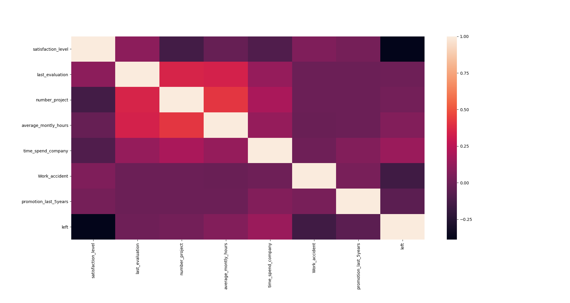
Highly correlated feature could be combined to form a new feature. In this case we may about combining average_montly_hours and number_project which have a correlation of 0.41. Instinctively it seems obvious that this 2 parameters are correlated. Still, I consider the correlation coefficient still quite low and decided to keep all the information.
numpy implementation of knn
Each of our individual in represented by 7 features. Let’s simplify the problem in order to understand how knn works and say that each of our example in represented by only 2 features. A representation of our dataset in the 2 dimensional space could be :
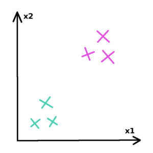
This is the database we are going to build our model on. In this example, 2 groups with different labels(green and pink) are clearly differentiated.
Let’s now introduce a new unlabeled employee for which we would like to predict if he will stay or leave the company. We can position it in our space.
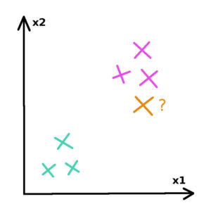
To which group does this new employee belongs?
In order to evaluate this knn propose to do as follow :
- calculate distance from new employee to every employee in the dataset
- select the k nearest employees (k minimum values of our table of distances)
- vote for the most represented label in the k nearest employees
To measure the distance between 2 employees, we choose the squared euclidean distance metric such as :
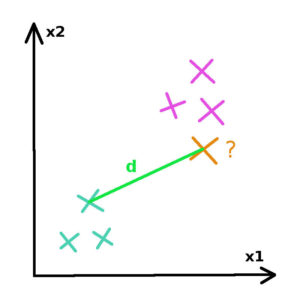
Each example is represented by x1 and x2 values. Let’s have two individuals a=(a1,a2) and b=(b1,b2), the euclidean distance between this 2 individuals can be calculated with the following formula :

function 1 : calculating the distance between 2 elements
|
1 2 3 4 |
#calculate the distance between 2 individuals def distance(ind1,ind2): distance=np.sum((ind1-ind2)**2) return distance |
function 2 : generating the distance table
We iterate through labeled data and calculate distance with new employee for each example in our dataset.
|
1 2 3 4 5 6 |
#create the table if distances between the new example and every other labelled data def kdistance(new_example,labelled_data): dist=[] for i in list(range(0,len(labelled_data))): dist.append(distance(new_example,labelled_data[i])) return dist |
function 3 : vote for the k nearest neighbors
The choice of k can be discussed. My advice about k:
- k should not be divisible by the number of different labels. In our example we have 2 groups of labels. So k should be an odd number. It will avoid the equal probabilities situations where our algorithm could not make a choice for prediction
- k should be smaller that the quantity of individual in the smallest group. My concern is that if 2 groups are close to each other, a small group may struggle to compete against a bigger neighbor group.
For this study, I choose k=5
|
1 2 3 4 5 6 |
def knn(k,kdistance_table): enum=np.argsort(kdistance_table)[:k]#get the k smallest values in the table of distance predictions=y_train[enum] c=Counter(predictions) key=[element for element, count in c.most_common(1)] #vote for the most common element in our predictions vector return key[0] |
function 4 : predictions and accuracy
We compare our predictions to our labelled data in the test dataset.
|
1 2 3 4 5 6 7 8 9 |
def accuracy(X_test,y_test,X_train): total=len(y_test) liste=[] for example in range(len(X_test)): prediction=knn(5,kdistance(X_test[example],X_train)) liste.append(prediction) good_predictions=np.sum(liste==y_test) accuracy=good_predictions/total return accuracy |
Results
We reach 95.8% of accuracy on our predictions.
|
1 |
accuracy of algorithm is 0.9586666666666667 |
Knn is a very simple algorithm that can perform quite well for a prestudy. It’s not as powerfull as other machine learning algorithm, but it ‘s easy to set up and does not require a lot of computation power.
This version of the algorithm is not optimized we still have pretty good results with it. Let’s implement the scikit-learn version of knn and compare the results with the same value of k=5.
|
1 2 3 4 5 6 7 8 9 10 11 12 13 14 15 16 |
#scikit-learn solution for knn clf=neighbors.KNeighborsClassifier() #k default value is 5 clf.fit(X_train,y_train) accuracy=clf.score(X_test,y_test) print(accuracy) new_example=np.array([0.10,0.1,10,150,7,0,0]) new_example=new_example.reshape(1,-1) prediction=clf.predict(new_example) if (prediction==1): p="leave the company" else: p="stay in the company" print("For individual with characteristics",new_example,"our prediction is that he will", p) |
Results
|
1 |
accuracy of algorithm is 0.9526666666666667 |
We have similar accuracy values, which confirms that our algorithm has been properly coded.
Resources
- http://scikit-learn.org/stable/index.html