Python : neural network

16/01/2017

Introduction

To code your own neural network is often the first great challenge each data scientist has to face. It’s a pretty good exercise to check that one has understood each step and process of training a simple neural network once it has been built. On this page I am going to describe the maths and the code I used to build a simple deep neural network.

Our target is to build a neural network which could digest any kind of standardized data. The design of the neural network is manageable by changing the number of layers and the quantity of neurons we want per layer.

The data for the example comes from this Kaggle’s competition. I only kept the numerical data to be injected in the network. The objective is to build a model which could predict which employee is about to leave a company for HR purposes. Therefore, on this page, I am obviously building a classification model.

The full code is available on Github.

Import dependencies

The aim of this exercise is to create a neural network class which will automatically train on your dataset. We will use the basic following libraries of python. Most of the algorithms of a neural network uses sum and multiplication of matrices.

#dependencies---------------------------------------------------------------------------------------

import numpy as np #matrix multiplication + maths
import pandas as pd #data management
import os #file system

#dependencies---------------------------------------------------------------------------------------

import numpy as np #matrix multiplication + maths

import pandas as pd #data management

import os #file system

Data Retrieving

My data is store as a csv file. I am using panda reader to load it into a variable called “data”.

#data retrieving------------------------------------------------------------------------------------
os.chdir("C:\\Users\\Nicolas\\Google Drive\\website\\python-own neuralnetwork")
data=pd.read_csv("data.csv",sep=";")

#m : number of exemples, p : numbers of features
m=data.shape[0]
p=data.shape[1]

#Separating Inputs and outputs ---------------------------------------------------------------------
X=data.ix[:,0:p-1] #not including p-1
y=data.iloc[:,p-1]
Yreal=[]
for i in range(len(y)):
	if y[i]==1:
		Yreal.append([1,0])
	elif y[i]==0:
		Yreal.append([0,1])

#data retrieving------------------------------------------------------------------------------------

os.chdir("C:\\Users\\Nicolas\\Google Drive\\website\\python-own neuralnetwork")

data=pd.read_csv("data.csv",sep=";")

#m : number of exemples, p : numbers of features

m=data.shape[0]

p=data.shape[1]

#Separating Inputs and outputs ---------------------------------------------------------------------

X=data.ix[:,0:p-1] #not including p-1

y=data.iloc[:,p-1]

Yreal=[]

for i in range(len(y)):

if y[i]==1:

Yreal.append([1,0])

elif y[i]==0:

Yreal.append([0,1])

We retrieve the data in a big dataframe (data) and then separate the inputs (features in X matrix) and the output (y matrix or vector). The output format is a vector of 2 elements for each example. In the original csv file, if the employee left the company then we have y=1 which I translate to Yreal=[1,0] (Yreal=[0,1] if he stayed).

Standardize Data

Our input matrix contains m examples. Each example (or individual) is represented by p parameters and has one y result that we would like to predict. So we can represent the data this way.

Input matrix X :

$\begin{bmatrix} X_{1}^{1} X_{2}^{1} ... X_{p}^{1}\\ X_{1}^{2} X_{2}^{2} ... X_{p}^{2} \\ ... \\ X_{1}^{m} X_{2}^{m} ... X_{p}^{m} \end{bmatrix}$

Output vector or matrix y :

$\begin{bmatrix} y^{1}\\ y^{2} \\ ... \\ y^{m} \end{bmatrix}$

Before we launch our prediction model calculation, we need to normalize the data. So let’s do it element wise for matrix X with the help of numpy. You will also find the definition of each variable that I’ll be using in the code.

#network definitions--------------------------------------------------------------------------------
# Z : output vector for each layer
# X : input vector for each layer
# W : Weights matrix
# a : values vector after applying the sigmoid function to Z, a becomes the new input vector for the next layer
# y : real value vector of the ouput
# yth : theoritical value vector calculated by our network
# e : error vector between y and yth
# J : costfunction, return single value

def normalize(X):
	return X/np.amax(X)

#network definitions--------------------------------------------------------------------------------

# Z : output vector for each layer

# X : input vector for each layer

# W : Weights matrix

# a : values vector after applying the sigmoid function to Z, a becomes the new input vector for the next layer

# y : real value vector of the ouput

# yth : theoritical value vector calculated by our network

# e : error vector between y and yth

# J : costfunction, return single value

def normalize(X):

return X/np.amax(X)

The maths and concept

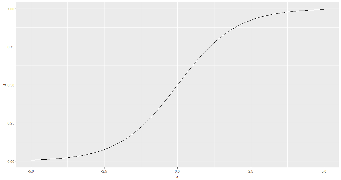
The first important notion in understanding a neural network is the activation function. The sigmoid function will activate (a=1) or deactivate (a=0) a neuron in our network. It will allow us to build logical functions between the network. It is defined as follows :

$(0) : sigmoid(z)=\frac{1}{1+e^{-z}}$

Here is what the function looks like :

def sigmoid(z):
	return 1.0/(1.0+np.exp(-z))

def softmax(z):
	softmax = np.exp(z-np.max(z))/np.sum(np.exp(z-np.max(z)),axis=1,keepdims=True)
	return softmax

def sigmoid(z):

return 1.0/(1.0+np.exp(-z))

def softmax(z):

softmax = np.exp(z-np.max(z))/np.sum(np.exp(z-np.max(z)),axis=1,keepdims=True)

return softmax

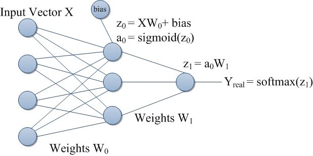
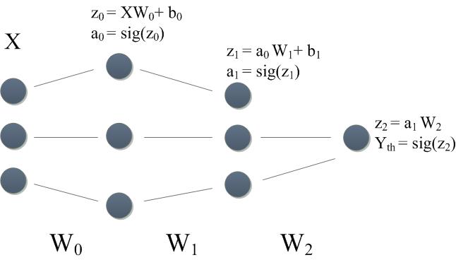
In a deep neural network, the data is processed during a process that we call forward propagation. For each layer we will switch neurons to on or off to adjust the response of the final output.

Now we are going to talk about the object we define as a “neuron”. This object simply transforms several input values into a new output value with the help of the sigmoid function. Let’s have a look at how it works.

We can define several elements in this object :

X : inputs of the neurons
W : weights of each branch of the neuron
Z : intermediate value of the calculus
A : activation, it is the final output of our neuron and it will define if our neuron is activated or not

Now let’s play with these. The rules are simple; we are going through the process of calculating the activation A with the following formulas :

$(1) : Z_{1}=\sum_{i=1}^{p} X_{i}W_{i}$

$(2) : A_{1}=sigmoid(Z_{1})=\frac{1}{1+e^{-Z_{1}}}$

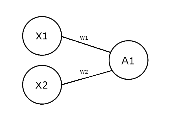
Building OR and AND logic gates :

Ok, let’s try to build 2 different kind of logic gates. The weights of the network can be either negative or positive. Depending on the combination of weights, we will be able to build different logic functions. Here are some examples :

X1	X2	W1	W2	Z1	A1
1	1	20	10	30	~1
0	0	20	10	0	~0.5
1	0	20	10	20	~1

Here we can notice one of the problems that we may encounter with a neural network, if the 2 inputs are close to zero, then the sigmoid function is not able to decide whether or not it needs to activate the following neurons. One of the ways to solve this is to add some bias to each layer of the network in order to force the decision in one direction (activated / deactivated).

So here is the design of the new network :

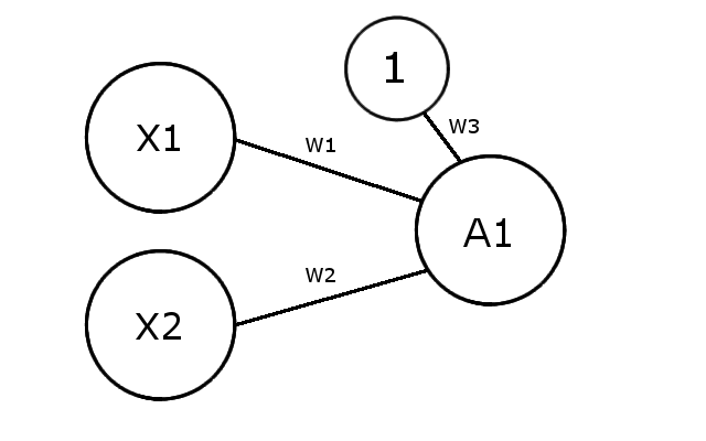
In order to create an AND gate, we would like our network to respect the following table :

X1	X2	X1 AND X2
1	1	1
0	0	0
1	0	0

which, if we translate into equations, gives us the following system :

$\left\{\begin{matrix}X_{1}W_{1}+X_{2}W_{2}+W_{3}>0 \\ W_{3}<0 \\ X_{1}W_{1}+W_{3}<0 \end{matrix}\right.$

A set of values for the weight W that answers this system could be

W=[W1,W2,W3]=[10,20,-20]

Using equations (1) and (2), let’s check if it answers to our system properly.

X1	X2	Bias	W1	W2	W2	Z1	A1
1	1	1	10	20	-20	10	~1
0	0	1	10	20	-20	-20	~0
1	0	1	10	20	-20	-10	~0

This weight vector W=[W1,W2,W3] is creating an AND logic gate. More complex logical functions are available in a neural network but they require more layers of neurons. Other non-linear relationships can be built through a neural network. Combination of these logical functions is what makes a neural network powerful regarding classification and regression tasks.

The OR weight matrix

Now let’s try to build an OR logic gate.

We need to propose a set of weights which answers :

X1	X2	X1 OR X2
1	1	1
0	0	0
1	0	1

which can be translated to the following system:
$\left\{\begin{matrix}X_{1}W_{1}+X_{2}W_{2}+W_{3}>0 \\ W_{3}<0 \\ X_{1}W_{1}+W_{3}>0 \end{matrix}\right.$

Compared to the AND system, only the last equation is changed. A vector of weights that could answer this system is W=[W1,W2,W3]=[30,10,-20].

X1	X2	Bias	W1	W2	W2	Z1	A1
1	1	1	30	10	-20	20	~1
0	0	1	30	10	-20	-20	~0
1	0	1	30	10	-20	10	~1

Our new set of weights matches our expectation. What we are going to do during the training phase of the neural network is to tweak the values of W to adjust the response of our system.

The NOT logical function is set regarding the sign of the weight. If the weight is negative, then positive inputs become negatives. It turns out that with these 3 logical functions only, we are able to create all possible existing logic gates.

We have enough knowledge about the concept and the maths to construct the first part of our algorithm. It will consist of processing the inputs through our network layer after layer, neurons after neurons until the value of the final output is determined. We call this process “Forward propagation”.

Initialize network architecture

In order to build a neural network, we need to process in 2 steps : forward propagation and cost reduction. In the very beginning of our code, we want to initialize some values that will characterize the network.

n_hidden : (single value) number of hidden layers
n_neurons : (vector) number of neurons per hidden layers

Inputs and the output of the neural network are defined by your data set (X and Yreal). As we have seen previously, networks are made of weights and bias. Before we begin our training, we would like to assign random values to our bias and weights. Let’s build the random functions.

def Weights(k,l):
	return np.random.randn(k,l)

def bias(l):
	return np.random.rand(l) #it is better to start with positive values for bias

def Weights(k,l):

return np.random.randn(k,l)

def bias(l):

return np.random.rand(l) #it is better to start with positive values for bias

Once I have defined the architecture of our network (qty of layers and qty of neurons per layer), I am creating all the weights and bias objects associated with each layer. For example if we have 2 hidden layers, we will create W={W[0],W[1],W[2]} and b={b[0],b[1],b[2]}.

def create_network(input,n_hidden,n_neurons,output):
	W=dict()
	b=dict()
	for i in range(n_hidden+1):
		if i==0:
			W[i]=Weights(input.shape[1],n_neurons[i])
			b[i]=bias(n_neurons[i])
		elif i==n_hidden:
			W[i]=Weights(n_neurons[i-1],2)
			b[i]=bias(2)
		else:
			W[i]=Weights(n_neurons[i-1],n_neurons[i])
			b[i]=bias(n_neurons[i])
	return W,b

def create_network(input,n_hidden,n_neurons,output):

W=dict()

b=dict()

for i in range(n_hidden+1):

if i==0:

W[i]=Weights(input.shape[1],n_neurons[i])

b[i]=bias(n_neurons[i])

elif i==n_hidden:

W[i]=Weights(n_neurons[i-1],2)

b[i]=bias(2)

else:

W[i]=Weights(n_neurons[i-1],n_neurons[i])

b[i]=bias(n_neurons[i])

return W,b

Forward propagation

We can now code the functions (1) and (2) that will apply the forward propagation to our algorithm. These functions will use the sigmoid function that we have defined previously. For each layer we propagate the inputs to the next layer using weights and biases.

def forward(input,W,b):
	for layer in range(len(W)):
		if layer==0:
			Yth=np.dot(input,W[layer])+b[layer]
			Yth=sigmoid(Yth)
		elif layer==len(W)-1:
			Yth=np.dot(Yth,W[layer])+b[layer]
			Yth=softmax(Yth)
		else:
			Yth=np.dot(Yth,W[layer])+b[layer]
			Yth=sigmoid(Yth)
	return Yth

def forward(input,W,b):

for layer in range(len(W)):

if layer==0:

Yth=np.dot(input,W[layer])+b[layer]

Yth=sigmoid(Yth)

elif layer==len(W)-1:

Yth=np.dot(Yth,W[layer])+b[layer]

Yth=softmax(Yth)

else:

Yth=np.dot(Yth,W[layer])+b[layer]

Yth=sigmoid(Yth)

return Yth

Cost Error calculation

Now that we could calculate our final output, we are able to quantify the error between the expected results and our calculated results. We will use a classic definition of cost (or error) J.

$(3) : J=\frac{1}{2m}\sum_{i=1}^{m} (Y_{th}-Y_{real})^{2}$

We are summing the error of all the examples of our training set. Then we will try to have a look at the importance of each weight layer regarding our error.

Translation to python :

def cost(Yth,Yreal):
	J=np.sum((Yth-Yreal)**2)/(2*len(Yreal))
	return J

def cost(Yth,Yreal):

J=np.sum((Yth-Yreal)**2)/(2*len(Yreal))

return J

Gradient Descent on cost (Backward propagation)

Finally we have reached the learning phase of our neural network. J is the function we would like to minimize (we want to minimize the error between real and predicted values), and we are going to do it the same way we do it since highschool. We will calculate the partial derivative of the J function and look for the zeros (using the gradient descent algorithm). How much does the cost vary regarding each layer of weight? It will help us to adjust the values of W in order to reduce J (we are finaly tuning the network).

As defined we have our cost value :

$(3) : J=\frac{1}{2m}\sum_{i=1}^{m} (Y_{th}-Y_{real})^{2}$

Let’s calculate the derivative value regarding W1 using simple derivative rules (f o g)’ = f'(g) . g’

$\frac{\partial J}{\partial W_{1}}=\frac{1}{2m}\sum_{i=1}^{m}\frac{\partial(Y_{th}-Y_{real})^{2} }{\partial W_{1}}$

$\frac{\partial J}{\partial W_{1}}= \frac{1}{2m}\sum_{i=1}^{m}2(Y_{th}-Y_{real})\frac{\partial Yth}{\partial W_{1}}$

$\frac{\partial J}{\partial W_{1}}= \frac{1}{m}\sum_{i=1}^{m}(Y_{th}-Y_{real})\frac{\partial Yth}{\partial W_{1}}$

We have $Yth = sigmoid(a_{0}W_{1}+b_{1})$ , so we can easily calculate the second term.

$\frac{\partial J}{\partial W_{1}}= \frac{1}{m}\sum_{i=1}^{m}(Y_{th}-Y_{real})\frac{\partial Y_{th}}{\partial Z_{1}}\frac{\partial Z_{1}}{\partial W_{1}}$

$\frac{\partial J}{\partial W_{1}}= \frac{1}{m}\sum_{i=1}^{m}(Y_{th}-Y_{real})\frac{e^{-Z_{1}}}{(1+e^{-Z_{1}})^2}a_{0}$

Now let’s try to calculate the derivative of J regarding the first weight layer W0. The calculation of the last term can be tricky for deep layers in your network. We need to decompose the calculation of this derivative using the chain rule.

$\frac {\partial y}{\partial x}=\frac {\partial y}{\partial u}.\frac {\partial u}{\partial x}$

$\frac{\partial J}{\partial W_{0}}=\frac{1}{2m}\sum_{i=1}^{m}\frac{\partial(Y_{th}-Y_{real})^{2} }{\partial W_{0}}$

$\frac{\partial J}{\partial W_{0}}= \frac{1}{m}\sum_{i=1}^{m}(Y_{th}-Y_{real})\frac{\partial Yth}{\partial W_{0}}$

Using chain rule, we have:

$\frac{\partial J}{\partial W_{0}}= \frac{1}{m}\sum_{i=1}^{m}(Y_{th}-Y_{real})\frac{\partial Yth}{\partial Z_{1}}.\frac{\partial Z_{1}}{\partial a_{0}}.\frac{\partial a_{0}}{\partial Z_{0}}.\frac{\partial Z_{0}}{\partial W_{0}}$

$\frac{\partial J}{\partial W_{0}}= \frac{1}{m}\sum_{i=1}^{m}(Y_{th}-Y_{real}).\frac{e^{-Z_{1}}}{(1+e^{-Z_{1}})^2}.W_{1}.\frac{e^{-Z_{0}}}{(1+e^{-Z_{0}})^2}.X$

We can now generalize for the gradient of J :

$(5) : \frac{\partial J}{\partial W_{j}}=\frac{1}{m}{}\sum_{i=1}^{m}(Y_{th}-Y_{real})\frac{\partial Y_{th}}{\partial W_{j}}$

$(5) : \frac{\partial J}{\partial W_{j}}=\frac{1}{m}{}\sum_{i=1}^{m}\left [ (Y_{th}-Y_{real})a_{j}\prod_{j}^{nhidden}dsigmoid(z_{j})\prod_{j+1}^{nhidden}W_{j+1}\right ]$

The first weights $W_0$ and the last Weights are kind of particular cases to this equation. For $W_0$ , $a_j$ will become $X$ . For the last $W$ (on the right of the neural network) there is no multiplication by any W (as $W_{j+1}$ does not exist).

Practically, to start our gradient descent we need to define a learning rate (the speed of the descent) and also the number of steps we want our algorithm to proceed.

Let’s first code the gradient calculation

def gradient(Yth,Yreal,X,J,W):
	gradient=dict()
	delta=dict()
	Z=dict()
	a=dict()
	for layer in range(len(W)):
		if layer==0:
			Z[layer]=np.dot(X,W[layer])
			a[layer]=sigmoid(Z[layer])
		else:
			Z[layer]=np.dot(a[layer-1],W[layer])
			a[layer]=sigmoid(Z[layer])


	for layer in reversed(range(len(W))):
		if layer==len(W)-1:
			delta[layer]=np.multiply((Yth-Yreal),dsigmoid(Z[layer]))
			gradient[layer]=np.dot(a[layer-1].transpose(),delta[layer])

		else:
			if layer==0:
				delta[layer]=np.dot(delta[layer+1],W[layer+1].transpose())*dsigmoid(Z[layer])
				gradient[layer]=np.dot(X.transpose(),delta[layer])
			else:
				delta[layer]=np.dot(delta[layer+1],W[layer+1].transpose())*dsigmoid(Z[layer])
				gradient[layer]=np.dot(a[layer-1].transpose(),delta[layer])


	return gradient,a

def gradient(Yth,Yreal,X,J,W):

gradient=dict()

delta=dict()

Z=dict()

a=dict()

for layer in range(len(W)):

if layer==0:

Z[layer]=np.dot(X,W[layer])

a[layer]=sigmoid(Z[layer])

else:

Z[layer]=np.dot(a[layer-1],W[layer])

a[layer]=sigmoid(Z[layer])

for layer in reversed(range(len(W))):

if layer==len(W)-1:

delta[layer]=np.multiply((Yth-Yreal),dsigmoid(Z[layer]))

gradient[layer]=np.dot(a[layer-1].transpose(),delta[layer])

else:

if layer==0:

delta[layer]=np.dot(delta[layer+1],W[layer+1].transpose())*dsigmoid(Z[layer])

gradient[layer]=np.dot(X.transpose(),delta[layer])

else:

delta[layer]=np.dot(delta[layer+1],W[layer+1].transpose())*dsigmoid(Z[layer])

gradient[layer]=np.dot(a[layer-1].transpose(),delta[layer])

return gradient,a

And finally perform our gradient descent :

def gradient_descent(gradient,W,b,learning_rate):
	for layer in range(len(W)):
		W[layer]=W[layer]-learning_rate*gradient[layer]
	return W

def gradient_descent(gradient,W,b,learning_rate):

for layer in range(len(W)):

W[layer]=W[layer]-learning_rate*gradient[layer]

return W

Now, we have to keep in mind that several issues may occur during this process. Gradient descent may struggle to find the global minimum of J and may get stuck in a local minimum.

$(6) : W_{i}=W_{i}-\alpha \frac{\partial J}{\partial W_{i}}$

Each weight layer is updated separately using its proper partial derivative. At this point it is often a good idea to check your numeric calculation by comparing the results of the derivative and a numerical estimation.

Training the network

We have built the complete model, now it’s time to train the network. For each epoch, we will perform gradient descent to minimize the error of our forward propagation (prediction).

#parameters-----------------------------------------------------------------------------------------
n_neurons=[4]
n_hidden=len(n_neurons)

#normalization of the inputs and network initialization---------------------------------------------
X=normalize(X)
W,b=create_network(X,n_hidden,n_neurons,y)
	
#Calculate 1st forward propagation and initial cost-------------------------------------------------
Yth=forward(X,W,b)

J=cost(Yth,Yreal)

learning_rate=0.0005

#training the network-------------------------------------------------------------------------------
for epoch in range (10000):
	Yth=forward(X,W,b)
	J=cost(Yth,Yreal)
	print('cost is : ',J)
	grad=gradient(Yth,Yreal,X,J,W)
	for layer in range(len(W)):
		W[layer]=gradient_descent(grad[layer],W[layer],b[layer],learning_rate)

#parameters-----------------------------------------------------------------------------------------

n_neurons=[4]

n_hidden=len(n_neurons)

#normalization of the inputs and network initialization---------------------------------------------

X=normalize(X)

W,b=create_network(X,n_hidden,n_neurons,y)

#Calculate 1st forward propagation and initial cost-------------------------------------------------

Yth=forward(X,W,b)

J=cost(Yth,Yreal)

learning_rate=0.0005

#training the network-------------------------------------------------------------------------------

for epoch in range (10000):

Yth=forward(X,W,b)

J=cost(Yth,Yreal)

print('cost is : ',J)

grad=gradient(Yth,Yreal,X,J,W)

for layer in range(len(W)):

W[layer]=gradient_descent(grad[layer],W[layer],b[layer],learning_rate)

Once the training is finished we have a ready-to-be-used model (weights and biases) for which we could feed any other new input. To save the model and use it later on, we just need to store weights, biases and the architecture of the network in a file on our computer.

Predictions and performance calculation

Here are some KPI we can use in order to assess the performance of our model on some project. Basically it consists of training your model on one part of your dataset (70 to 80%) and checking on the remaining labelled data if your classifier is working properly. We can then build the confusion matrix from our experiments.

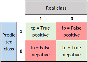
We can have a look to the following indicator :

$Accuracy = \frac{tp+tn}{Total}$

$Precision = \frac{tp}{tp + fp}$

$Recall = \frac{tp}{tp+fn}$

$F1score = 2\frac{Precision*Recall}{Precision+Recall}$

Conclusion

That’s it for my understanding of neural networks and how to code one from scratch in python. It may not be the latest technique, but I hope this article could help you to have a better understanding of how we build this kind of object and what the underlying mathematics are. There are many more things to implement in this deep neural network code, such as overfitting solutions (regularization, dropout,…).

More complex network architectures such as convolutional neural networks or recurrent neural networks are way more difficult to code from scratch. Hopefully, some professional programmers have coded more advanced tools around neural network, and I personally use libraries for R and python in my studies (R : neuralnet, python 3.5 : tensorflow).

Github python neural network

Sources of inspirations for this page

http://www.welchlabs.com/ and its wonderful youtube channel.

http://cs229.stanford.edu/ machine learning course from Stanford

https://www.coursera.org/learn/machine-learning/home machine learning course from Stanford by Andrew Ng (video)