16/01/2017

Tensorflow I : newbie level

For a more advanced machine learning classifier, it is a good idea to use the powerful tool that Google released in 2016. Tensorflow is optimized and built to solve your most complex data project. In this article, I will be discovering this library and trying to apply it to small examples. This discovery process of the tool is very important in order to be able to scale up on a bigger project. On this page, we are going to code a deep neural network in python using the Tensorflow library. Our target is to be able to easily change the design (number of layers and neurons per layer) by just changing some variables in the code.

Before we begin, here is the link to latest version of the code : Github

Installing the library along with python 3.5 and Windows

In the command line of windows

pip install tensorflow

1	pip install tensorflow

Please note, that it will install the CPU version of Tensorflow. If you would like to use GPUs to make your calculation you will need to install another version of Tensorflow and configure your system to work along with Tensorflow.

Loading the library

import tensorflow as tf

1	import tensorflow as tf

Building the datasets

For the first exercise we would like to build a classifier that would be able to tell the difference between cats and dogs in pictures. The data comes from the kaggle website. In the “dog vs cat” challenge, they propose a dataset composed of 25 000 labelled pictures.

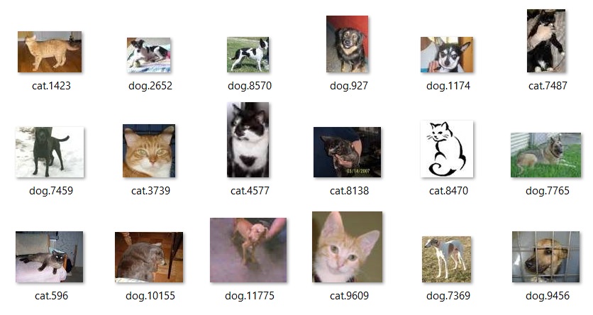
Each picture has different dimensions. I would like to focus only on the model building part, so I will implement a very simple treatment of the pictures for standardization.

Croping, resizing and greying the pictures

I would like all the pictures to have the same size : 120×120 pixels. The following piece of code is not efficient at all. All the pictures are cropped to the center, meaning that if the animal does not have its face in the center, we may lose a lot of information.

tocrop function : transform any picture into a squared picture using the current min dimension

def tocrop(list):
        dim=[]
        for file in list:
                img=Image.open(file)
                min=np.min(img.size)
                img=ImageOps.fit(img,(min,min),Image.ANTIALIAS)
                img.save('C:/Users/Nicolas/Google Drive/website/python-tensorflow/croptrain/' + file,"JPEG")

def tocrop(list):

dim=[]

for file in list:

img=Image.open(file)

min=np.min(img.size)

img=ImageOps.fit(img,(min,min),Image.ANTIALIAS)

img.save('C:/Users/Nicolas/Google Drive/website/python-tensorflow/croptrain/' + file,"JPEG")

tothumb function : reduce the size to our desired dimension : 120×120 pixels. Smaller pictures will not be able to size up. I chose to filter them out when we feed our model.

def tothumb(list):
	dim=[]
	for file in list:
		img=Image.open(file)
		dim.append(img.size)
	
	for file in list:
		img=Image.open(file)
		img.thumbnail([120,120],Image.ANTIALIAS)
		img.save('C:/Users/Nicolas/Google Drive/website/python-tensorflow/thumbtrain/' + file,"JPEG")

def tothumb(list):

dim=[]

for file in list:

img=Image.open(file)

dim.append(img.size)

for file in list:

img=Image.open(file)

img.thumbnail([120,120],Image.ANTIALIAS)

img.save('C:/Users/Nicolas/Google Drive/website/python-tensorflow/thumbtrain/' + file,"JPEG")

togrey function : just convert colored image to greyscale picture

def togrey(list):
	for file in list:
		img=Image.open(file)
		img=img.convert('L')
		img.save('C:/Users/Nicolas/Google Drive/website/python-tensorflow/greytrain/'+file,"JPEG")

def togrey(list):

for file in list:

img=Image.open(file)

img=img.convert('L')

img.save('C:/Users/Nicolas/Google Drive/website/python-tensorflow/greytrain/'+file,"JPEG")

Using these 3 functions, I finally have my “standardized” input pictures. As said, this is clearly not the best way to do it, as I may have lost a lot of information, but I would say that for most pictures we can still see a cat or dog face on the image.

Dependencies

#Building the classifier with Tensorflow

import os
import csv
import matplotlib
import tensorflow as tf
from numpy import array
import numpy as np
from PIL import Image

#Building the classifier with Tensorflow

import os

import csv

import matplotlib

import tensorflow as tf

from numpy import array

import numpy as np

from PIL import Image

I will use the following listed dependencies :

os : to navigate through the system, list files, etc…
csv : to generate csv files (result file)
matplotlib : to display charts or pics
tensorflow : the machine learning library
numpy : for math operations
PIL : image reading and saving

Loading input and output data

We would like to create a deep neural network. For those who do not know, deep neural networks look like this :

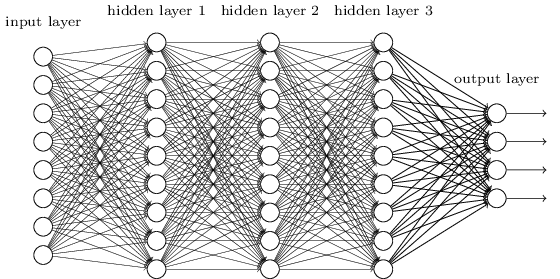
We will inject our pictures in the input layer and receive an answer (“dog” or “cat”) on the output layer after propagation of the data through the hidden layers.

#import images and flatten it into a array (examples x flatten_pixels)

train="\\python-tensorflow\\greytrain"
os.chdir(train)
list=os.listdir()
input=[]
output=[]
y_dog=[0,1]
y_cat=[1,0]

#building input array (examples, flatten image)
for file in list :
	img=Image.open(file)
	arr=array(img)
	if arr.shape[0]==120:
		flat=arr.flatten()
		input.append(flat)
		if "cat" in file:
			output.append(y_cat)
		elif "dog" in file:
			output.append(y_dog)

input=np.array(input)
input.astype('float32')

output=np.asarray(output)
print(input.shape)
print(output.shape)

#import images and flatten it into a array (examples x flatten_pixels)

train="\\python-tensorflow\\greytrain"

os.chdir(train)

list=os.listdir()

input=[]

output=[]

y_dog=[0,1]

y_cat=[1,0]

#building input array (examples, flatten image)

for file in list :

img=Image.open(file)

arr=array(img)

if arr.shape[0]==120:

flat=arr.flatten()

input.append(flat)

if "cat" in file:

output.append(y_cat)

elif "dog" in file:

output.append(y_dog)

input=np.array(input)

input.astype('float32')

output=np.asarray(output)

print(input.shape)

print(output.shape)

We create 2 empty lists : input and output. Input is fed with flattened images. We flatten the 2D pictures into a 1D vector. Only pictures with dimension 120*120 are selected. The output array is made of cat [1,0] and dog [0,1] vectors and is built with the name of the file (which contains the labels). Lists are then transformed to numpy arrays type.

Finally we can check the size of each array to be sure that everything is ok. In my case :

input : (24588,14400). 120×120 pixels = 14 400 flatten pixels
output : (24588,2)

While filtering image dimension, we only removed 412 pictures from our set. We still have a nice quantity of data to train our network.

A good idea is to normalize the input data. It will help our model to converge during the training phase. We are using standard normalization and we apply it image by image.

$X=\frac{X-\mu }{\sigma }$

input=(input-np.mean(input,axis=0))/np.std(input,axis=0)

1	input=(input-np.mean(input,axis=0))/np.std(input,axis=0)

Building the network

We have a lot of tasks to achieve in this part. I will build all the layers manually, but I know there are some functions in Tensorflow that allow you to do it more properly.

Let’s first declare the shape of our network.

#design of network
n_neurons=[124,15] #neurons for each hidden layer
n_hidden=len(n_neurons)

#design of network

n_neurons=[124,15] #neurons for each hidden layer

n_hidden=len(n_neurons)

In n_neurons, we can declare any vector of any length. It is a representation of the hidden layers. Each value represents the quantity of neurons we have for each layer.

From the previous information we can build the entire network with the following function. It will return us lists of weights and biases.

def network_shape(input,ouput,n_hidden,n_neurons):
	with tf.name_scope("Layers"):
		global W #yeah I know this is bad ^^
		global b
		W=dict()
		b=dict()
		for i in range(1,n_hidden+2):
			if i==1:
				W[i]=Weights(input.shape[1],n_neurons[i-1])
				b[i]=bias(n_neurons[i-1])
			elif i==n_hidden+1:
				W[i]=Weights(n_neurons[i-2],output.shape[1])
				b[i]=bias(output.shape[1])
			else:
				W[i]=Weights(n_neurons[i-2],n_neurons[i-1])
				b[i]=bias(n_neurons[i-1])
	return W,b

def network_shape(input,ouput,n_hidden,n_neurons):

with tf.name_scope("Layers"):

global W #yeah I know this is bad ^^

global b

W=dict()

b=dict()

for i in range(1,n_hidden+2):

if i==1:

W[i]=Weights(input.shape[1],n_neurons[i-1])

b[i]=bias(n_neurons[i-1])

elif i==n_hidden+1:

W[i]=Weights(n_neurons[i-2],output.shape[1])

b[i]=bias(output.shape[1])

else:

W[i]=Weights(n_neurons[i-2],n_neurons[i-1])

b[i]=bias(n_neurons[i-1])

return W,b

Each of the weight and bias arrays are initialized with the following functions :

#Create my Weights matrices and Bias vector for each layer of the NN 
def Weights(k,l):
	with tf.name_scope("Weights"):
		W=tf.Variable(tf.truncated_normal([k,l],stddev=0.1),name='Weights')
	return W

def bias(l):
	with tf.name_scope("bias"):
		b=tf.Variable(tf.truncated_normal([l],stddev=0.1),name="bias")
	return b

#Create my Weights matrices and Bias vector for each layer of the NN

def Weights(k,l):

with tf.name_scope("Weights"):

W=tf.Variable(tf.truncated_normal([k,l],stddev=0.1),name='Weights')

return W

def bias(l):

with tf.name_scope("bias"):

b=tf.Variable(tf.truncated_normal([l],stddev=0.1),name="bias")

return b

Weights and biases are initialized with random values distributed along a Gaussian model with standard deviation of 0.1.

Building the model

We can now define our model. The forward propagation is defined as follows :

def multilayer(X,W,b):
	Yth=X
	for layer in range(1,len(W)+1):
		if layer!=len(W):
			Yth=tf.nn.relu(tf.matmul(Yth,W[layer])+b[layer])
		else:
			Yth=tf.nn.softmax(tf.matmul(Yth,W[layer])+b[layer])
	return Yth

Yth=multilayer(X,W,b) #performing forward propagation with an input matrix and a neural network (Weights + biases)

def multilayer(X,W,b):

Yth=X

for layer in range(1,len(W)+1):

if layer!=len(W):

Yth=tf.nn.relu(tf.matmul(Yth,W[layer])+b[layer])

else:

Yth=tf.nn.softmax(tf.matmul(Yth,W[layer])+b[layer])

return Yth

Yth=multilayer(X,W,b) #performing forward propagation with an input matrix and a neural network (Weights + biases)

We use a “relu” activation function for the hidden layers and a “softmax” activation function for the last layer. Our output will appear as statistics (level of confidence for each picture to represent a dog or a cat).

Cost function definition : we will use cross entropy to evaluate our loss.

cross_entropy = tf.reduce_mean(tf.nn.softmax_cross_entropy_with_logits(logits=Yth, labels=Yreal))

1	cross_entropy = tf.reduce_mean(tf.nn.softmax_cross_entropy_with_logits(logits=Yth, labels=Yreal))

Gradient descent

train_step = tf.train.GradientDescentOptimizer(learning_rate).minimize(cross_entropy,global_step=global_step)

1	train_step = tf.train.GradientDescentOptimizer(learning_rate).minimize(cross_entropy,global_step=global_step)

Decaying learning rate

global_step=tf.Variable(0,trainable=False)
starter_learning_rate=0.15
learning_rate=tf.train.exponential_decay(starter_learning_rate,global_step,1000,0.5)

global_step=tf.Variable(0,trainable=False)

starter_learning_rate=0.15

learning_rate=tf.train.exponential_decay(starter_learning_rate,global_step,1000,0.5)

Our learning rate starts at 0.15 and will decay by 50% every 1000 epochs. I totally randomly chose these values.

Placeholders

Tensorflow needs a placeholder for input and labels to be defined. We will use it to feed our model during the training phase.

X = tf.placeholder(tf.float32, [None,input.shape[1]],name='X')
Yreal = tf.placeholder(tf.float32, [None,output.shape[1]],name='Yreal')

1 2	X = tf.placeholder(tf.float32, [None,input.shape[1]],name='X') Yreal = tf.placeholder(tf.float32, [None,output.shape[1]],name='Yreal')

Preparing sets

permutation = np.random.permutation(input.shape[0]) #shuffling the rows
input=input[permutation]
output=output[permutation]
train_set=input[0:int(0.8*input.shape[0])]
train_label=output[0:int(0.8*input.shape[0])]
test_set=input[int(0.8*input.shape[0])+1:input.shape[0]]
test_label=output[int(0.8*output.shape[0])+1:output.shape[0]]

permutation = np.random.permutation(input.shape[0]) #shuffling the rows

input=input[permutation]

output=output[permutation]

train_set=input[0:int(0.8*input.shape[0])]

train_label=output[0:int(0.8*input.shape[0])]

test_set=input[int(0.8*input.shape[0])+1:input.shape[0]]

test_label=output[int(0.8*output.shape[0])+1:output.shape[0]]

In this part, I am shuffling my input and output dataset (permutations) and separate the entire set in 2 subsets : 80% of the data is going to the training set, 20% of the data is going to a test set.

Training the network

#session start
sess = tf.Session()
sess.run(init)

for epoch in range(0,2000):
	permutation=np.random.permutation(19600)
	permutation=permutation[0:1200]
	batch=[train_set[permutation],train_label[permutation]]
	_,loss_val=sess.run([train_step,cross_entropy],feed_dict={X:batch[0],Yreal:batch[1]})
	print("epoch" ,epoch ,"is being processed")
	print(loss_val,W[1].eval(session=sess))

#session start

sess = tf.Session()

sess.run(init)

for epoch in range(0,2000):

permutation=np.random.permutation(19600)

permutation=permutation[0:1200]

batch=[train_set[permutation],train_label[permutation]]

_,loss_val=sess.run([train_step,cross_entropy],feed_dict={X:batch[0],Yreal:batch[1]})

print("epoch" ,epoch ,"is being processed")

print(loss_val,W[1].eval(session=sess))

We are training our model by batch. Every epoch a random batch is created with 1200 inputs and labels then being fed to Tensorflow. I am printing the loss value in order to check if our model is converging or not and if we can reach zero loss for our training set.

Performance assessment

We can assess the performance of our algorithm by measuring its accuracy.

#accuracy on the test set
correct_prediction = tf.equal(tf.argmax(Yth,1), tf.argmax(Yreal,1))
accuracy = tf.reduce_mean(tf.cast(correct_prediction, tf.float32))
prediction=Yth
print(sess.run(prediction, feed_dict={X: test_set, Yreal: test_label}))
print(sess.run(accuracy, feed_dict={X: test_set, Yreal: test_label}))

#accuracy on the test set

correct_prediction = tf.equal(tf.argmax(Yth,1), tf.argmax(Yreal,1))

accuracy = tf.reduce_mean(tf.cast(correct_prediction, tf.float32))

prediction=Yth

print(sess.run(prediction, feed_dict={X: test_set, Yreal: test_label}))

print(sess.run(accuracy, feed_dict={X: test_set, Yreal: test_label}))

With a single hidden layer of 124 neurons and by playing a little bit with learning rate and batch size value, I could achieve a 65% accurate prediction rate,… which is really bad .

Conclusions

It’s only taken a few minutes to compute the results. There are several ways to improve the performance of the model. We could have treated the input images more carefully, keep the color information, or applied Principal Component algorithm. Playing with the design of the neural network is usually a good idea but adding more layers tends to make overfitting appear (the model has some difficulty to generalize). In the next chapter, I am going to try to set up a convolutional neural network which seems more adequate for image classification. Let’s go further with Tensorflow!

Go to Tensforflow II : intermediate level