Dataset for this study : UCI
Datasets is composed of different clients (columns) for which a measurement of electric consumption has been recorded every 15 min for years. I expect to witness seasonality and trend in the signal. I’ll try to figure it out and build a regression model on it. This article aim to be an introduction to data analysis of time series.
Loading data and dependencies
|
1 2 3 4 5 6 7 8 9 10 11 12 13 14 15 16 17 18 19 20 21 22 23 24 |
import numpy as np import pandas as pd import matplotlib.pyplot as plt import os from autocorrelation import autocorrelate from scipy.fftpack import fft from scipy import signal #load data data=pd.read_csv('LD2011_2014.txt',sep=";") print(data.shape) #first column is the timestamp #every other column represent a customer #convert data to proper types data.iloc[:,0]=pd.to_datetime(data.iloc[:,0]) data.iloc[:,1]=pd.to_numeric(data.iloc[:,1].str.replace(',','.')) #client1 prestudy client1=data.iloc[:,0:2] client1.columns=['timestamp','consumption'] client1.head() |
Time series
Time series data are a particular form of signal type data. Usually, time series consists of a sequence of measurements. In most simple cases, every data point is recorded on a regular time basis, but usually we will be facing non regular sequences dataset. Here are 2 examples of regular and irregular time series :
- A thermometer sensor is linked to a computer, the computer records the temperature every hour.
- A sportsman is using a sportapp, which can record its activities.
a. Scalar product on time series : signal decomposition
Each basis must be composed with unitary vectors, and each vector must be orthogonal. We can verify these properties with the computation of the magnitude of each vector (norm of vector = 1) and the two by two scalar product of each vector in the basis.
b. Dimension of a signal
Dimension of a signal is the quantity of parameters that have an effect on the signal.
c. Mean value

|
1 |
mean=sum(signal)/len(signal) |
d. Rms value
While mean value can be null, we would like to be able to describe the amplitude of the signal. Rms value is one way to do it :

|
1 |
rms=np.sqrt(np.dot(signal,signal)/len(signal)) |
e. Energy of a signal
Depends on the amplitude and the length (number of points) of the signal.

|
1 |
energy=np.dot(signal,signal) |
f. Power of a signal
Square of the rms value.

|
1 |
power=energy/len(signal) |
g. Euclidean distance between 2 signals
2 signals with the same dimension represented in the same space can be compared using the euclidean distance. This value is difficult to interpret, but is often used to compare it to another euclidean distance. It’s a good tool to evaluate the performance of our models and compare them.

|
1 |
euclidean=np.sqrt(sum((signal1-signal2)**2)) |
h. decomposition and recomposition of a signal (projection on a basis)
A signal can be decomposed on an orthonormal basis. Let’s build an orthogonal basis made of several sinus signals.
Resampling
It’s unlikely that our time serie is distributed evenly with constant gap between 2 following points. Resampling techniques allows to decrease or increase the number of time steps in the serie and more important to make it with a regular distribution. Different rules can apply to calculate the missing values (mean, max, min, etc…).
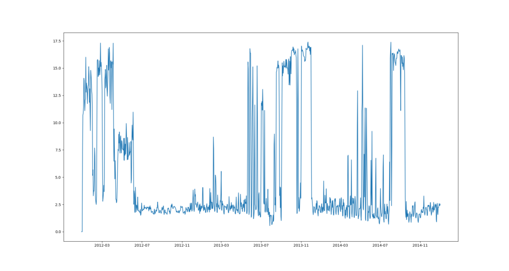
Let’s resample our data to daily
|
1 2 3 4 5 6 7 |
client1=client1.set_index('timestamp') #resampling client1_daily=client1.resample('D').mean() #ploting values plt.plot(client1_daily) plt.show() |
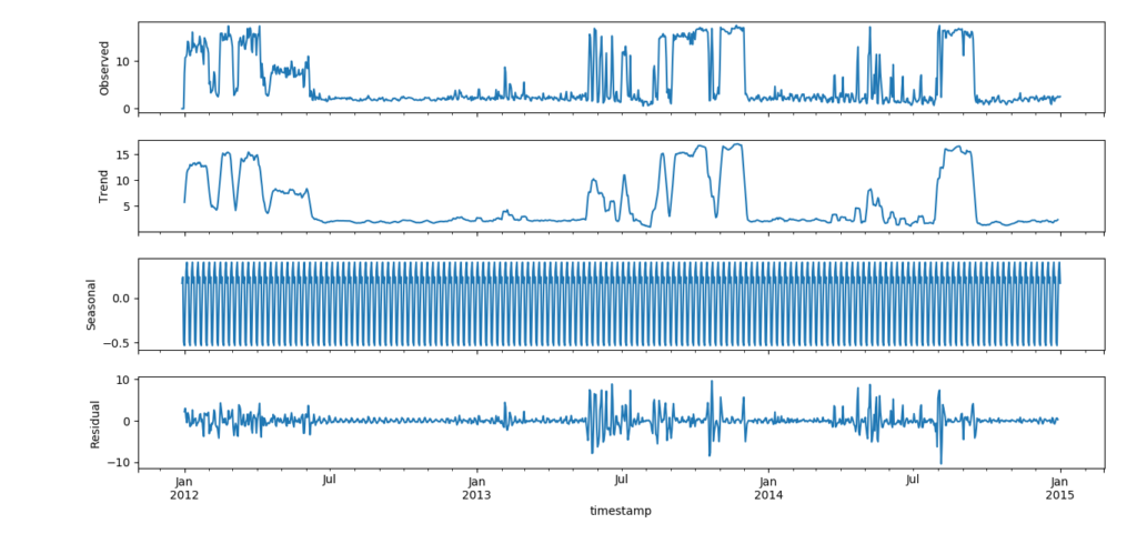
additive or multiplicative model?
Observed signals can be decomposed in 3 components : trend signal, seasonality signal, and noise signal.
|
1 2 3 4 5 6 7 8 9 10 11 |
from statsmodels.tsa.seasonal import seasonal_decompose result = seasonal_decompose(series, model='additive') print(result.trend) print(result.seasonal) print(result.resid) print(result.observed) result.plot() plt.show() |
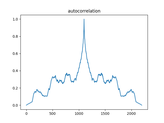
autocorrelation
|
1 2 |
#autocorrelation acr=autocorrelate(client1_flat) |
Frequency domain
a. Change of basis. Fourier basis (f1 to fn)
Construction of the basis

b. Signal decomposition in Fourier basis
Transformation of a signal u in the Fourier basis is given by the scalar product of u with the conjugate complex of each vector from the Fourier basis.
![TF[u]_{n}=\sum_{0}^{N-1}u_{k}e^{-j2\pi\frac{n}{N}k}](https://smalldatabrains.com/wp-content/ql-cache/quicklatex.com-5430e44cce6f4d568c716fd53df6e671_l3.png "Rendered by QuickLaTeX.com")
Fourier transform is a complex number.
c. Spectrogram
Spectrum is the module of the Fourier transform
N : length of our signal
We begin by building the Fourier basis Fn, composed of N vectors. We then check that our basis is “almost” an orthogonal basis by calculating the dot product value of vectors 2 by 2 and comparing it to a threshold value.
Finally, decomposition of the signal u is given by the dot product of u with the conjugate of Fn vectors.
|
1 2 3 4 5 6 7 8 9 10 11 12 13 14 15 16 17 18 19 20 21 22 23 24 25 26 27 28 29 30 31 32 33 34 35 36 37 38 39 40 41 42 43 44 45 46 47 48 49 50 |
#Fourier transform of a 1d signal import numpy as np import math import matplotlib.pyplot as plt x=np.arange(0,300) u=np.sin(x)*x+np.cos(x*2) plt.plot(x,u) plt.show() #let u be our signal N=len(u) k=np.arange(0,N) Fn=[] freq=[] #Fourier basis for n in range(0,N): f=np.exp(1j*2*math.pi*n/N*k) Fn.append(f) freq.append(n/N) print(len(Fn)) print(len(freq)) #check orthogonality of the fourier basis for f in range(len(Fn)): other=[x for i,x in enumerate(Fn) if i!=f] for l in range(len(other)): dot=np.dot(Fn[f],other[l]) if dot>0.000001: #checking if the scalar is small print(l,"th and",f,"th vectors are not orthogonal") print("scalar product value is",dot) print("False") TF=[] #decomposition in Fourier basis for f in range(len(Fn)): tfu=np.dot(u,Fn[f].conjugate()) TF.append(tfu/N) #ploting of the spectrum module=np.absolute(TF) plt.plot(freq,module,'--o',ms=3) #comparison with built in function plt.plot(freq,abs(np.fft.fft(u))/N) plt.show() |
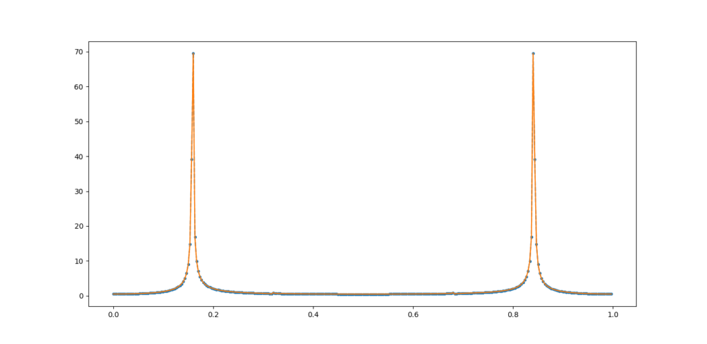
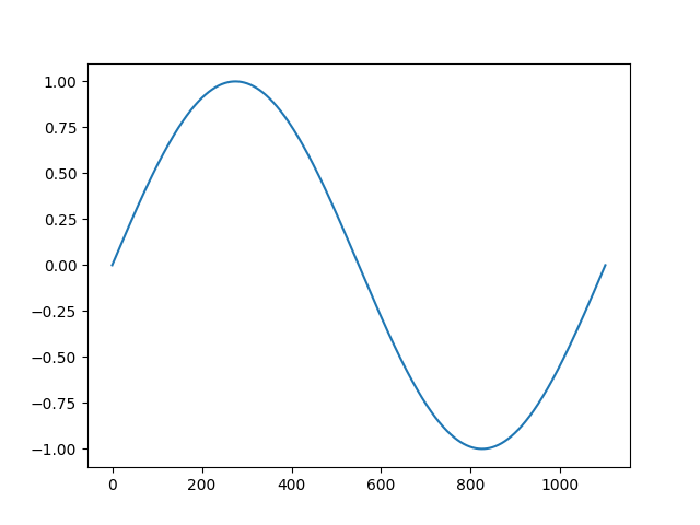
in blue, our Fourier function, in orange the one included in numpy. We can see that the values are matching, which validate our algorithm.
d. Convolution of 2 signals
Convolution is an operation which transform 2 signals (u1,u2) into an output signal (s) such as :

We often write convolution as follow :
s = u1 * u2 = u2 * u1
e. smoothing signal with convolution
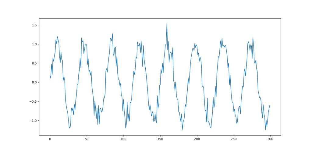
Let’s define a noisy signal as follow.
|
1 2 3 4 |
x=np.arange(0,300) y=np.sin(x/6)+np.random.randn(300)/6 plt.plot(x,y) plt.show() |
We want to use convolution to smooth the signal. Let’s start by averaging the signal with a small window.

We can write this equation as a convolution of the signal u with a gate signal such as :

Forecasting series with LSTM
LSTM networks can be usde to predict the next output of a serie given the previous inputs. In the following, I am just going to describe a simple implementation of such a model.
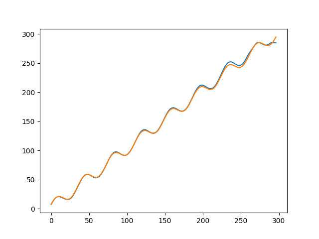
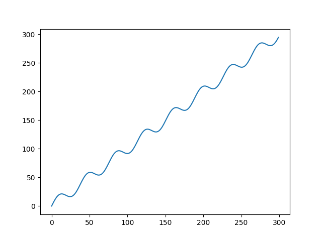
We are going to predict a sinus signal with a trend defined as follow :
|
1 2 3 4 5 6 |
#data x=np.arange(0,300) y=10*np.sin(x/6)+x plt.plot(x,y) plt.show() |
Given a number of previous time steps, we would like to predict the output of the signal. We need to define some parameters and to prepare the data so it could be fed properly into an LSTM keras layer.
Our signal contains len(x)=300 inputs points. Given the previous 10 points, we are going to predict the value of the next point.
|
1 2 3 4 5 |
#parameters input_size=len(x) print("There are",input_size,"entries in our serie") time_steps=10 batch_size=200 |
Preparation of the data.
The network will be fed with 10 inputs (time_steps) and 1 output. For each window of ten values in our serie we are going to send to the network a vector containing the values of the window (inputs) and the following value just after our window (ouput or label).
|
1 2 3 4 5 6 7 8 9 10 11 12 13 14 15 16 17 |
#data prepatation for neural network inputs=[] labels=[] time_steps=3 for i in range(0,input_size-time_steps,1): X_buffer=y[i:i+time_steps] y_buffer=y[i+time_steps] inputs.append(X_buffer) labels.append(y_buffer) inputs=np.asarray(inputs) labels=np.asarray(labels) print("inputs has shape",inputs.shape) print("labels has shape",labels.shape) inputs=np.reshape(inputs,(inputs.shape[0],1,inputs.shape[1])) |
Now that pairs of inputs and label are ready, we can feed it into the network.
Building and training the model in Keras.
I choose a LSTM network with one hidden layer of 50 neurons.
|
1 2 3 4 5 6 7 8 |
#building the network model=Sequential() model.add(LSTM(50,input_shape=(inputs.shape[1],inputs.shape[2]))) model.add(Dense(1)) model.compile(loss="mae",optimizer="adam") #training history=model.fit(inputs,labels,epochs=15000,batch_size=batch_size,verbose=1,shuffle=False) |
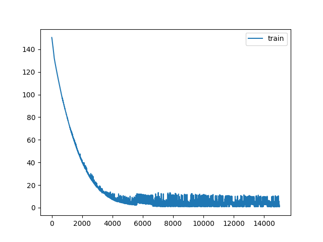
Plot the loss on the training set.
Loss on training set has a nice decreasing curve. Our network is learning properly.
|
1 2 3 4 |
#visualization of the results plt.plot(history.history['loss'],label='train') plt.legend() plt.show() |
Make the prediction.
|
1 2 3 4 5 |
#predictions Ypred=model.predict(inputs) plt.plot(Ypred) plt.plot(labels) plt.show() |